What is Linear Regression?:- Linear Regression is a Machine learning algorithm that identifies the relationship between a dependent variable and an independent variable. It works by drawing a regression line i.e. y=mx+c. Where,

y - dependent variable

m- a slope of the line.

x - Independent variable

c - Y-intercept

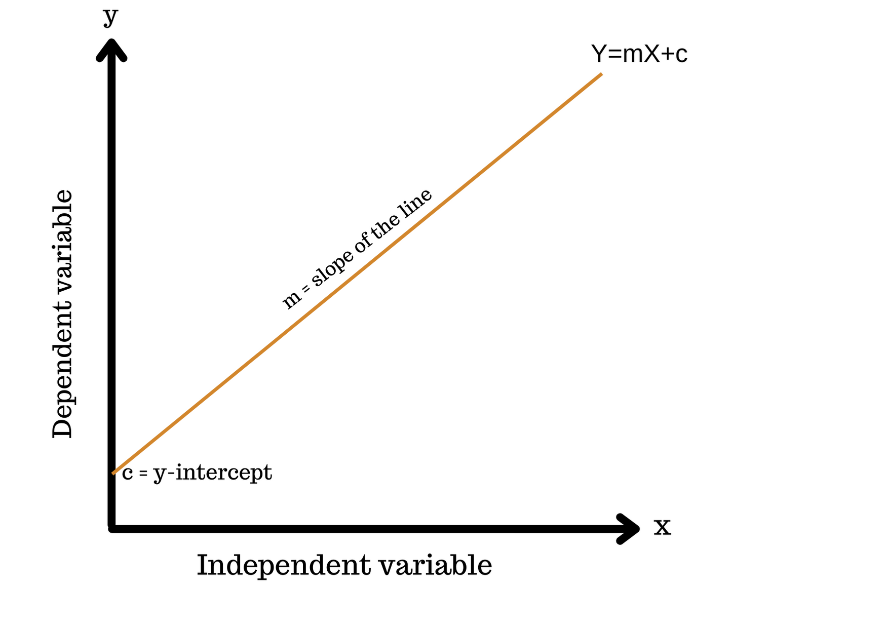
Here, If the dependent variable increases with the increase of the independent variable then the regression line will be positive. If the dependent variable decreases with the increase of the independent variable then the regression line will be negative.

Let's code.

x = [1,2,3,4,5]
y = [3,4,2,4,5]

X=sum(x)/len(x) #mean of x
Y=sum(y)/len(y) #mean of y

here, the value of X will be 3 and Y will be 4 which are nothing but the means. Now, we know we have the equation of the line, y=mx+c.

so, our next step is to find the value of m. So, here we have the formula to find the value of m.

m = Σ(x-X) (y-Y) / (x-X)*(x-X)

We are just taking the summation of all the values of x and y after subtracting it from their respective means.

for i in range(len(x)):
    s1+=(x[i]-X)*(y[i]-Y)
    s2+=(x[i]-X)*(x[i]-X)
m=s1/s2

Now, when we have the value of x,y and m let's find the value of c. If y=mx+c then, c=Y-mx

c = Y-(m*X)   #where Y and X are means
print("The value of m is: ",m)
print("The value of c is: ",c)

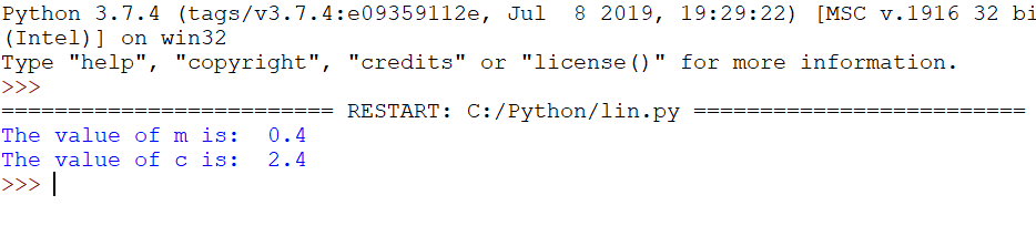
Here, the value of m is 0.4, and the value of c is 2.4 Now, the equation will be y=0.4x+2.4 now we will predict the values for y for every value of x.

y_predicted=[]
for i in range(len(x)):
    yP=(m*x[i])+c
    y_predicted.append(yP)
print("The values of Y is: ",y)
print("The values of Y predicted is: ",y_predicted)

Here is the output:-

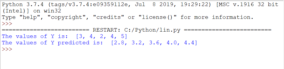
As we can see, the error rate is very high. Now let's find the value of R^2.

What is R squared?

R squared value is a statistical measure of how close the data points are to the fitted regression line.

R2 = ∑(y_predicted - Y)^2 / ∑(y - Y)^2

up=[]
low=[]
s=0
for i in range(len(y_predicted)):
   s=y_predicted[i]-Y
   up.append(s*s)
s=0
for i in range(len(y)):
   s=y[i]-Y
   low.append(s*s)
R2=sum(up)/sum(low)
print("The value of R^2 is: ",R2)

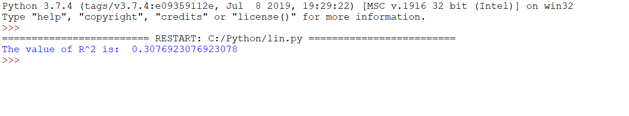Here, the value of R^2 is: 0.3

Let's plot a graph now.

from matplotlib import pyplot as plt
plt.plot(x,y,'rx')
plt.plot(x,y_predicted,'bx')
plt.grid()
plt.show()

Here is the output:-

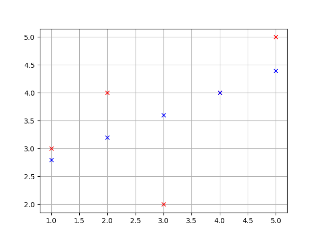
As you can see, the error rate is very high when the value of R^2 is 0.3. Here, red points are showing the values of y and blue points are showing the predicted values of y.

Now, using gradient descent, we will try to reduce the error rate as much as possible. Here, when the R^2 is 0.3, the error rate is a little high. So, the error rate can be reduced by toggling the value of R^2.

Here is the full code:-

x = [1,2,3,4,5]
y = [3,4,2,4,5]

X=sum(x)/len(x) 
Y=sum(y)/len(y)

s1=0
s2=0
for i in range(len(x)):
    s1+=(x[i]-X)*(y[i]-Y)
    s2+=(x[i]-X)*(x[i]-X)
m=s1/s2

c = Y- (m*X)  

y_predicted=[]
for i in range(len(x)):
    yP=(m*x[i])+c
    y_predicted.append(yP)

up=[]
low=[]
s=0
for i in range(len(y_predicted)):
    s=y_predicted[i]-Y
    up.append(abs(s))

up=[]
low=[]
s=0
for i in range(len(y_predicted)):
   s=y_predicted[i]-Y
   up.append(s*s)
s=0
for i in range(len(y)):
   s=y[i]-Y
   low.append(s*s)
R2=sum(up)/sum(low)
print("The value of R^2 is: ",R2)

from matplotlib import pyplot as plt
plt.plot(x,y,'rx')
plt.plot(x,y_predicted,'bx')
plt.grid()
plt.show()

In the next post, we will learn about Gradient Descent and try to increase the accuracy of our algorithm by decreasing the error rate.

Until then, show some love in the comment section.